Take Home Ex 2

Published

December 6, 2023

Modified

December 16, 2023

Overview of the Exercise

What are the driving forces behind urban dwellers to weak up early in morning to commute from their home locations to their work places? What are the impact of removing a public bus service on the commuters reside along the corridor of the bus route? These and many other questions related to urban mobility are challenges faced by transport operators and urban managers.

To provide answer to this question, traditionally, commuters survey will be used. However, commuters survey is a very costly, time-consuming and laborous, not to mention that the survey data tend to take a long time to clean and analyse. As a result, it is not unusual, by the time the survey report was ready, most of the information already out-of-date!

As city-wide urban infrastructures such as public buses, mass rapid transits, public utilities and roads become digital, the data sets obtained can be used as a framework for tracking movement patterns through space and time. This is particularly true with the recent trend of massive deployment of pervasive computing technologies such as GPS on the vehicles and SMART cards used by public transport commuters.

Unfortunately, this explosive growth of geospatially-referenced data has far outpaced the planner’s ability to utilize and transform the data into insightful information thus creating an adverse impact on the return on the investment made to collect and manage this data.

This take-home exercise is motivated by two main reasons. Firstly, despite increasing amounts of open data available for public consumption, there has not been significant practice research carried out to show how these disparate data sources can be integrated, analysed, and modelled to support policy making decisions.

Secondly, there is a general lack of practical research to show how geospatial data science and analysis (GDSA) can be used to support decision-making.

Hence, your task for this take-home exercise is to conduct a case study to demonstrate the potential value of GDSA to integrate publicly available data from multiple sources for building a spatial interaction models to determine factors affecting urban mobility patterns of public bus transit.

Open Gov Data

For the purpose of this assignment, data from several open government sources will be used:

Passenger Volume by Origin Destination Bus Stops, Bus Stop Location, Train Station and Train Station Exit Point, just to name a few of them, from LTA DataMall.
Master Plan 2019 Subzone Boundary, HDB Property Information, School Directory and Information and other relevant data from Data.gov.sg.
Added the data of childcare services obtained from onemap.gov.sg

Specially collected data

Businesses, retail and services, leisure and recreation, etc geospatial data sets assemble by course instructor. (Refer to eLearn)

The specific tasks of this take-home exercise are as follows:

Derive an analytical hexagon data of 375m (this distance is the perpendicular distance between the centre of the hexagon and its edges) to represent the traffic analysis zone (TAZ).

With reference to the time intervals provided in the table below, construct an O-D matrix of commuter flows for a time interval of your choice by integrating Passenger Volume by Origin Destination Bus Stops and Bus Stop Location from LTA DataMall. The O-D matrix must be aggregated at the analytics hexagon level

Peak hour period	Bus tap on time	What it Means (Likely)
*Weekday morning peak*	*6am to 9am*	*Going to work and school (our data will be focused on this)*
Weekday afternoon peak	5pm to 8pm	Returning home from work or school
Weekend/holiday morning peak	11am to 2pm	Heading out for retail shopping, attractions etc
Weekend/holiday evening peak	4pm to 7pm	Returning home for Mon Blues

Display the O-D flows of the passenger trips by using appropriate geovisualisation methods (not more than 5 maps).
Describe the spatial patterns revealed by the geovisualisation (not more than 100 words per visual).
Assemble at least three propulsive and three attractiveness variables by using aspatial and geospatial from publicly available sources.
Compute a distance matrix by using the analytical hexagon data derived earlier.

Spatial Interaction Modelling

Calibrate spatial interactive models to determine factors affecting urban commuting flows at the selected time interval.
Present the modelling results by using appropriate geovisualisation and graphical visualisation methods. (Not more than 5 visuals)
With reference to the Spatial Interaction Model output tables, maps and data visualisation prepared, describe the modelling results. (not more than 100 words per visual).

Getting Started

So for the purpose of this exercise - I will focus on the Weekdays Morning Travel Period.

I will also utilise the writing and loading of rds to reduce the rendering and loading time as well as make the site more reproducible.

Loading the Packages

pacman::p_load(tmap, sf, sp, DT,
               performance, reshape2,
               ggpubr, tidyverse, stplanr, jsonlite)

Preparing the Flow Data

#|eval: false

odbus <- read_csv("data/aspatial/origin_destination_bus_202310.csv")

#|eval: false
odbus6_9 <- odbus %>%
  filter(DAY_TYPE == "WEEKDAY") %>%
  filter(TIME_PER_HOUR >= 6 &
           TIME_PER_HOUR <= 9) %>%
  group_by(ORIGIN_PT_CODE,
           DESTINATION_PT_CODE) %>%
  summarise(TRIPS = sum(TOTAL_TRIPS))

#|eval: false
busstops = st_read(dsn = "data/geospatial", 
               layer = "BusStop") %>%
  st_transform (crs = 3414)

Reading layer `BusStop' from data source 
  `C:\zjjgithubb\ISSS624\TakehomeEx\Ex02\data\geospatial' using driver `ESRI Shapefile'
Simple feature collection with 5161 features and 3 fields
Geometry type: POINT
Dimension:     XY
Bounding box:  xmin: 3970.122 ymin: 26482.1 xmax: 48284.56 ymax: 52983.82
Projected CRS: SVY21

Create analytical hexagon data of 325m (this distance is the perpendicular distance between the centre of the hexagon and its edges) - so should be c(750, 750).

#|eval: false
hexagon_grid = st_make_grid(busstops, c(750, 750), what = "polygons", square = FALSE)

hexagon_grid_sf = st_sf(hexagon_grid) %>%
  mutate(grid_id = 1:length(lengths(hexagon_grid)))

#|eval: false
hexagon_grid_sf$n_busstops = lengths(st_intersects(hexagon_grid_sf, busstops))

hexagon_busstop = filter(hexagon_grid_sf, n_busstops > 0)

busstop_grid <- st_intersection(busstops, hexagon_grid_sf)%>%
  select(BUS_STOP_N, grid_id) %>%
  st_drop_geometry()

#|eval: false
od_data_wdam <- left_join(odbus6_9 , busstop_grid,
            by = c("ORIGIN_PT_CODE" = "BUS_STOP_N")) %>%
  rename(ORIGIN_BS = ORIGIN_PT_CODE,
         ORIGIN_Grid = grid_id,
         DESTIN_BS = DESTINATION_PT_CODE)

#|eval: false
duplicate <- od_data_wdam %>%
  group_by_all() %>%
  filter(n()>1) %>%
  ungroup()

#|eval: false
od_data_wdam <- unique(od_data_wdam)

#|eval: false
od_data_wdam <- left_join(od_data_wdam , busstop_grid,
            by = c("DESTIN_BS" = "BUS_STOP_N")) 

duplicate <- od_data_wdam %>%
  group_by_all() %>%
  filter(n()>1) %>%
  ungroup()

od_data_wdam <- unique(od_data_wdam)

od_data_wdam <- od_data_wdam %>%
  rename(DESTIN_Grid = grid_id) %>%
  drop_na() %>%
  group_by(ORIGIN_Grid, DESTIN_Grid) %>%
  summarise(MORNING_PEAK = sum(TRIPS))

#Removing Intra-Grid Flow
od_wdam_cleaned <- od_data_wdam[od_data_wdam$ORIGIN_Grid!=od_data_wdam$DESTIN_Grid,]

Write/Read Data into rds for Subsequent Usage

Code

write_rds(hexagon_busstop, "data/rds/hexagon_busstop.rds")

write_rds(od_wdam_cleaned, "data/rds/od_wdam_cleaned.rds")

write_rds(hexagon_grid_sf, "data/rds/hexagon_grid_sf.rds")

Code

hexagon_bustops <- read_rds("data/rds/hexagon_busstop.rds")

od_wdam_cleaned <- read_rds("data/rds/od_wdam_cleaned.rds")

hexagon_grid_sf <- read_rds("data/rds/hexagon_grid_sf.rds")

schools_sf <- read_rds("data/rds/schools_sf.rds")

mpsz <- read_rds("data/rds/mpsz.rds")

flow_data_tidy <- read_rds("data/rds/flow_data_tidy.rds")

Visualising the Spatial Interaction

Code

flowLine <- od2line(flow = od_wdam_cleaned, 
                    zones = hexagon_grid_sf,
                    zone_code = "grid_id")

Code

tmap_options(check.and.fix = TRUE)
tmap_mode("plot")

tm_shape(mpsz) +
  tm_polygons(col = "black", alpha = 0.5) +
  tm_layout(main.title = "Spatial Flow for Passengers by Bus on Weekdays Morning",
            main.title.position = "center",
            main.title.size = 1.0,
            frame = TRUE) +
  tm_borders(alpha = 0.5) +
  tm_compass(type="8star", size = 2) +
  tm_scale_bar() +
  tm_grid(alpha =0.2, labels.show = FALSE)+
tm_shape(hexagon_bustops) +
  tm_polygons(alpha = 0.3, col = "lightblue") +
flow_data_tidy %>%  
  filter(TRIPS >= 5000) %>%
tm_shape() +
  tm_lines(lwd = "TRIPS",
           style = "quantile",
           scale = c(0.1, 1, 3, 5, 7, 10),
           n = 6,
           col = "yellow",
           alpha = 0.5)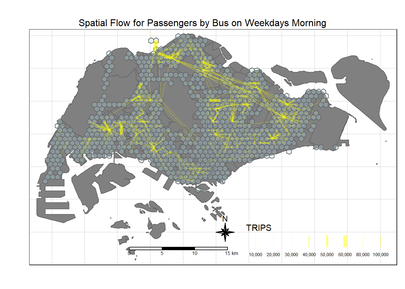

Code

tmap_options(check.and.fix = TRUE)
tmap_mode("plot")

tm_shape(mpsz) +
  tm_polygons(col = "black", alpha = 0.5) +
  tm_layout(main.title = "Spatial Flow for Passengers by Bus on Weekdays Morning, Dist > 10km",
            main.title.position = "center",
            main.title.size = 1.0,
            frame = TRUE) +
  tm_borders(alpha = 0.5) +
  tm_compass(type="8star", size = 2) +
  tm_scale_bar() +
  tm_grid(alpha =0.2, labels.show = FALSE)+
tm_shape(hexagon_bustops) +
  tm_polygons(alpha = 0.3, col = "lightblue") +
flow_data_tidy %>%  
  filter(TRIPS>=5000, DIST >= 10000) %>%
tm_shape() +
  tm_lines(lwd = "TRIPS",
           style = "quantile",
           scale = c(0.1, 1, 3, 5, 7, 10),
           n = 6,
           col = "yellow",
           alpha = 0.5)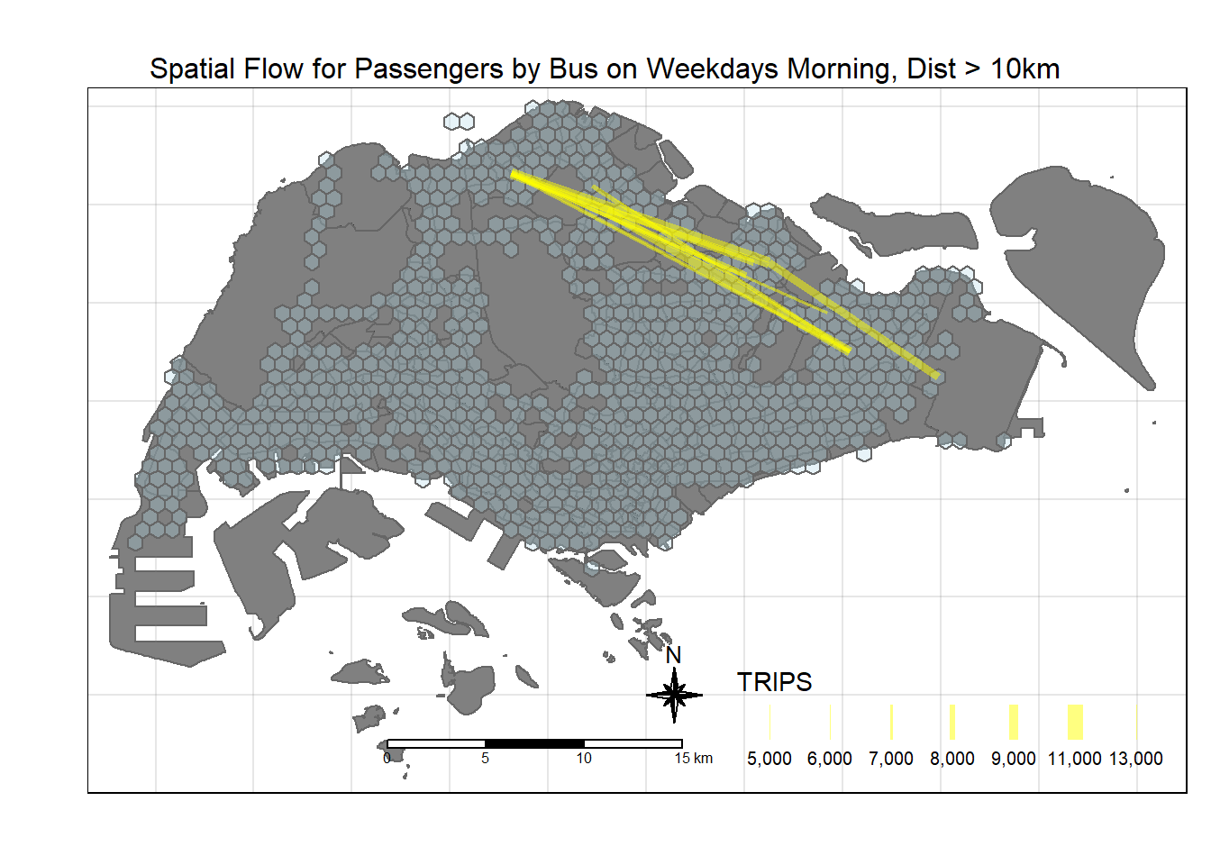

Analysis of Spatial Flow

From the spatial flow, it seems that there are a few identified areas where people are taking buses to during the morning peak period:

Travelling from Malaysia to Singapore through the Causeway - which accounts for a very high number. And it seems they will make their way towards Woodlands and branch out from that region.
Other regions include areas like Yishun, Tampines, Jurong, Boon Lay.
There are some long distances travel between Woodlands towards Changi, i.e. from the North to the Eastern Part of Singapore. This is probably due to a lack of direct MRT Lines, and that the Buses travelling on the Expressway would provide a speedier route.

Spatial Patterns

Attractiveness Variables

We will compile three attractiveness variables, namely:

Schools (their place of study)
Business (their place of work)
F&B (to buy breakfast before heading to their final destination, assuming that they will buy food nearer to their location)
Financial Services (locations about the banks and money changers in Singapore - assuming that people will travel there to work in the morning)

hexagon_bustops$SCHOOL_COUNT <- lengths(
  st_intersects(
    hexagon_bustops, schools_sf))

sum(hexagon_bustops$SCHOOL_COUNT)

We assume that the businesses equate to the companies etc that people will travel to for their work.

business_sf <- st_read(dsn = "data/geospatial", 
               layer = "Business")

business_sf<- unique(business_sf)

hexagon_bustops$BIZ_COUNT <- lengths(
  st_intersects(
    hexagon_bustops, business_sf))

food_sf <- st_read(dsn = "data/geospatial", 
               layer = "F&B") %>%
  st_transform (crs=3414)

food_sf<- unique(food_sf)

hexagon_bustops$FOOD_COUNT <- lengths(
  st_intersects(hexagon_bustops, food_sf))

finserv_sf <- st_read(dsn='data/geospatial',
                  layer='FinServ') %>% 
  st_transform(crs=3414)

finserv <- unique(finserv_sf)

hexagon_bustops$FINSERV_COUNT <- lengths(
  st_intersects(hexagon_bustops, finserv_sf))

Propulsive Variables

We will look at three propulsive variables, namely:

Number of Population
Number of Train Stations Exits
Number of Bus Stops (already available since Take Home Ex 1)
Location of Pre Schools (assuming parents will bring their child to the nearest pre-school which should be within walking distance, before going to the nearest bus stop to travel for work)
Number of Buses available within each grid - tried to obtain the bus route data from LTA Data Mall, but there data seems limited and outdated (no actual date on when it was last updated); so decided not to pursue this.

Preparing the Data on Populace

We utilise the hdb data provided by Prof.

hdb <- read_csv ("data/aspatial/hdb.csv")

Based on the data, we will be able to intersect the locations, types of dwellings (whether 1-room, 2-room, rental and etc) to have an estimate on the number of population in each grid.

So based on past studies in 2018:

Types of Dwelling	Average Household Size	Remarks
1-Room / Rental	2.3
2-Room	2.19
3-Room	2.63
4-Room	3.42
5-Room / Exec	3.77

hdb_tidy <- hdb %>%
  select(13:25, "lat", "lng") %>%
  mutate(one_Rm = (`1room_sold` + `1room_rental` + studio_apartment_sold + other_room_rental)*2.3) %>%
  mutate(two_Rm = (`2room_sold` + `2room_rental`)*2.19) %>%
  mutate(three_Rm = (`3room_sold` + `3room_rental`)*2.63) %>%
  mutate(four_Rm = (`4room_sold`) * 3.42) %>%
  mutate(five_rm = (`5room_sold` + `exec_sold` + multigen_sold)*3.77)

hdb_tidy <- hdb_tidy %>%
  select (14:20) %>%
  mutate (pop = one_Rm + two_Rm + three_Rm + four_Rm + five_rm)

Covert to sf data.

hdb_sf <- st_as_sf(hdb_tidy,
                      coords = c("lng", "lat"),
                      crs = 4326) %>%
  st_transform (crs=3414)

write_rds (hdb_sf, "data/rds/hdb_sf.rds")

hexagon_bustops$POP <- sapply(
  st_intersects(hexagon_bustops, hdb_sf),
  function(indices) sum(hdb_sf$pop[indices])
)

Train Station Exit

I think that the train station exits can be considered as both propulsive and attractive, e.g. people will take buses to the nearest train station exit, then take on the mrt to their next destination.

But they can also exit from the train station, then proceed to take bus to their place of work or study.

I downloaded the static shp file of the train station exits from LTADataMall.

train_exits_sf <- st_read(dsn = "data/geospatial", 
               layer = "Train_Station_Exit_Layer") %>%
  st_transform (crs=3414)

hexagon_bustops$TRAIN_EXITS_COUNT <- lengths(
  st_intersects(
    hexagon_bustops, train_exits_sf))

Location of Pre-Schools

Using the Onemap API, I gain access to the “Child Care Services” theme.

This is updated by ECDA in Dec 23 and i saved it in JSON format.

I will use the jsonlite package to convert the data.

childcare <- fromJSON("data/aspatial/childcare.json", flatten = TRUE)

childcare_tidy <- childcare %>%
  select(9:14) %>%
  slice(-1) %>%
  separate(col = SrchResults.LatLng, into = c("lat", "long"), sep = ",", convert = TRUE)

childcare_sf <- st_as_sf(childcare_tidy,
                      coords = c("long", "lat"),
                      crs = 4326) %>%
  st_transform (crs=3414)

hexagon_bustops$CHILDCARE_COUNT <- lengths(
  st_intersects(
    hexagon_bustops, childcare_sf))

All the data were combined and written into an rds file.

write_rds (hexagon_bustops, "data/rds/combined_data.rds")

combined_data <- read_rds("data/rds/combined_data.rds")

Visualising the Flow with the Variables

Code

tmap_options(check.and.fix = TRUE)
tmap_mode("plot")

tm_shape(mpsz) +
  tm_polygons(col = "grey", alpha = 0.5) +
  tm_layout(main.title = "Spatial Flow for Passengers by Bus on Weekdays Morning",
            main.title.position = "center",
            main.title.size = 1.0,
            frame = TRUE) +
  tm_borders(alpha = 0.5) +
  tm_compass(type="8star", size = 2) +
  tm_scale_bar() +
  tm_grid(alpha =0.2, labels.show = FALSE)+
tm_shape(combined_data[combined_data$SCHOOL_COUNT > 1, ]) +
  tm_borders() +
    tm_fill("SCHOOL_COUNT", alpha = 0.3) +
flow_data_tidy %>%  
  filter(TRIPS>=5000) %>%
tm_shape() +
  tm_lines(lwd = "TRIPS",
           style = "quantile",
           scale = c(0.1, 1, 3, 5, 7, 10),
           n = 6,
           col = "yellow",
           alpha = 0.5)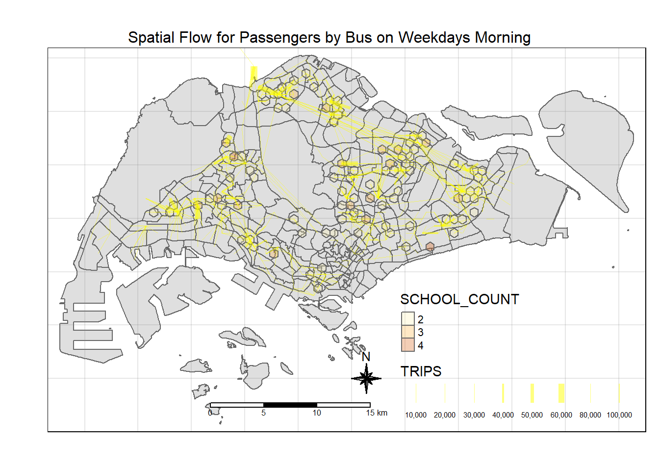

Code

tmap_options(check.and.fix = TRUE)
tmap_mode("plot")

tm_shape(mpsz) +
  tm_polygons(col = "grey", alpha = 0.5) +
  tm_layout(main.title = "Spatial Flow for Passengers by Bus on Weekdays Morning",
            main.title.position = "center",
            main.title.size = 1.0,
            frame = TRUE) +
  tm_borders(alpha = 0.5) +
  tm_compass(type="8star", size = 2) +
  tm_scale_bar() +
  tm_grid(alpha =0.2, labels.show = FALSE)+
tm_shape(combined_data[combined_data$SCHOOL_COUNT > 1, ]) +
  tm_borders() +
    tm_fill("BIZ_COUNT", alpha = 0.3) +
flow_data_tidy %>%  
  filter(TRIPS>=5000) %>%
tm_shape() +
  tm_lines(lwd = "TRIPS",
           style = "quantile",
           scale = c(0.1, 1, 3, 5, 7, 10),
           n = 6,
           col = "yellow",
           alpha = 0.5)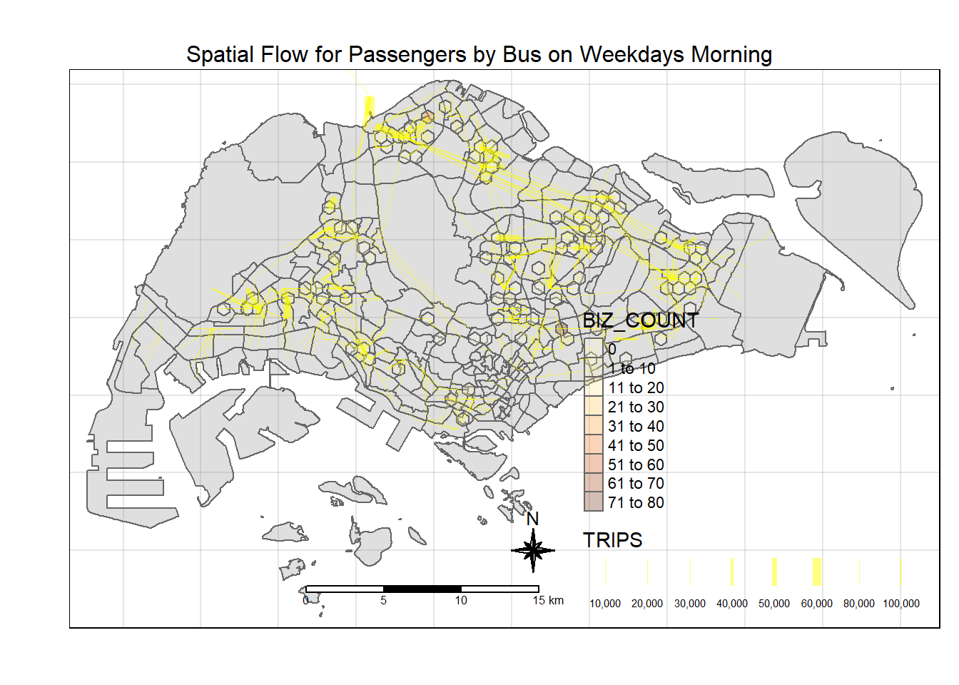

Code

tmap_options(check.and.fix = TRUE)
tmap_mode("plot")

tm_shape(mpsz) +
  tm_polygons(col = "grey", alpha = 0.5) +
  tm_layout(main.title = "Spatial Flow for Passengers by Bus on Weekdays Morning",
            main.title.position = "center",
            main.title.size = 1.0,
            frame = TRUE) +
  tm_borders(alpha = 0.5) +
  tm_compass(type="8star", size = 2) +
  tm_scale_bar() +
  tm_grid(alpha =0.2, labels.show = FALSE)+
tm_shape(combined_data[combined_data$SCHOOL_COUNT > 1, ]) +
  tm_borders() +
    tm_fill("POP", alpha = 0.3) +
flow_data_tidy %>%  
  filter(TRIPS>=5000) %>%
tm_shape() +
  tm_lines(lwd = "TRIPS",
           style = "quantile",
           scale = c(0.1, 1, 3, 5, 7, 10),
           n = 6,
           col = "yellow",
           alpha = 0.5)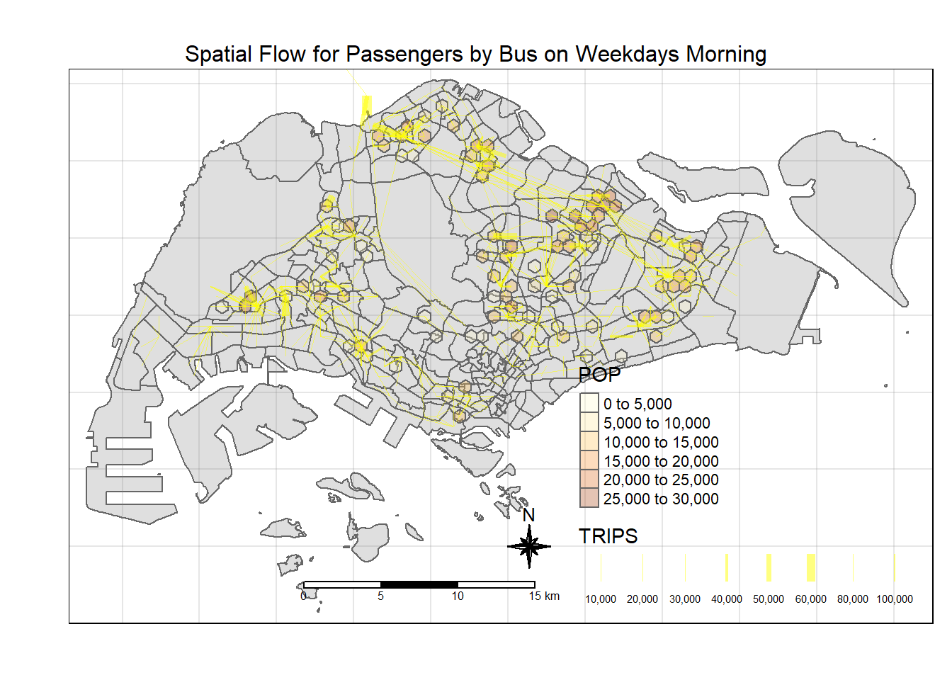

Spatial Interaction Modelling

Computing the Distance Matrix

hexa_sp <- as(hexagon_busstop,"Spatial")  
hexa_sp

dist <- spDists(hexa_sp,                  
                longlat = FALSE) #latlong is FALSE cuz its is in Svy21 alr  
head(dist, n=c(10, 10))

hexa_id <- hexagon_busstop$grid_id

colnames(dist) <- paste0(hexa_id) rownames(dist) <- paste0(hexa_id)

distPair <- melt(dist) %>%   rename(dist = value) head(distPair, 10)

distPair$dist <- ifelse(distPair$dist == 0,                         
                        50, distPair$dist)

distPair <- distPair %>%   rename(orig = Var1,          
                                  dest = Var2)

write_rds(distPair, "data/rds/distPair.rds")

distPair <- read_rds("data/rds/distPair.rds")

Preparing the Flow Data

Grouping the Flow Data

flow_data <- od_wdam_cleaned %>%
  group_by(ORIGIN_Grid, DESTIN_Grid) %>% 
  summarize(TRIPS = sum(MORNING_PEAK))

flow_data <- od2line(flow = flow_data, 
                    zones = hexagon_grid_sf,
                    zone_code = "grid_id")

Separating the Intra-Flow Data

flow_data$FlowNoIntra <- ifelse(
  flow_data$ORIGIN_Grid == flow_data$DESTIN_Grid, 
  0, flow_data$TRIPS)
flow_data$offset <- ifelse(
  flow_data$ORIGIN_Grid == flow_data$DESTIN_Grid, 
  0.000001, 1)

Combining Passenger Volume Data with Dist Data

flow_data1 <- flow_data %>%
  left_join (distPair,
             by = c("ORIGIN_Grid" = "orig",
                    "DESTIN_Grid" = "dest"))

Combining the Data with Propulsive and Attractive Variables Data

combined_tidy <- combined_data %>%
  st_drop_geometry()

combined_tidy$DESTIN_TRAIN_EXITS <- combined_tidy$TRAIN_EXITS_COUNT

flow_data_tidy <- flow_data1 %>%
  left_join(
    combined_tidy %>% 
      select(grid_id, SCHOOL_COUNT, BIZ_COUNT, FINSERV_COUNT, FOOD_COUNT, DESTIN_TRAIN_EXITS),
      by = c("DESTIN_Grid" = "grid_id")
  ) %>%
  rename(DIST = dist)

flow_data_tidy <- flow_data_tidy %>%
  left_join(
    combined_tidy %>% 
      select(grid_id, POP, TRAIN_EXITS_COUNT, CHILDCARE_COUNT, n_busstops),
      by = c("ORIGIN_Grid" = "grid_id")
  )

Ensure variables with value = 0 are adjusted to 0.99.

Code

flow_data_tidy$SCHOOL_COUNT <- ifelse(
  flow_data_tidy$SCHOOL_COUNT == 0,
  0.99, flow_data_tidy$SCHOOL_COUNT)

flow_data_tidy$BIZ_COUNT <- ifelse(
  flow_data_tidy$BIZ_COUNT == 0,
  0.99, flow_data_tidy$BIZ_COUNT)

flow_data_tidy$FINSERV_COUNT <- ifelse(
  flow_data_tidy$FINSERV_COUNT == 0,
  0.99, flow_data_tidy$FINSERV_COUNT)

flow_data_tidy$FOOD_COUNT <- ifelse(
  flow_data_tidy$FOOD_COUNT == 0,
  0.99, flow_data_tidy$FOOD_COUNT)

flow_data_tidy$TRAIN_EXITS_COUNT <- ifelse(
  flow_data_tidy$TRAIN_EXITS_COUNT == 0,
  0.99, flow_data_tidy$TRAIN_EXITS_COUNT)

flow_data_tidy$DESTIN_TRAIN_EXITS <- ifelse(
  flow_data_tidy$DESTIN_TRAIN_EXITS == 0,
  0.99, flow_data_tidy$DESTIN_TRAIN_EXITS)

flow_data_tidy$POP <- ifelse(
  flow_data_tidy$POP == 0,
  0.99, flow_data_tidy$POP)

flow_data_tidy$CHILDCARE_COUNT <- ifelse(
  flow_data_tidy$CHILDCARE_COUNT == 0,
  0.99, flow_data_tidy$CHILDCARE_COUNT)

write_rds (flow_data_tidy, "data/rds/flow_data_tidy.rds")

Calibrating Spatial Interaction Models

flow_data_tidy <- read_rds ("data/rds/flow_data_tidy.rds")

We will calibrate separate Spatial Interaction Models for inter- and intra-zonal flows. For the Ex, we will focus our attention on inter-zonal flow. Hence, we need to exclude the intra-zonal flow from flow_data.

First, two new columns called FlowNoIntra and offset will be created by using the code chunk below.

flow_data_tidy$FlowNoIntra <- ifelse(
  flow_data_tidy$ORIGIN_Grid == flow_data_tidy$DESTIN_Grid, 
  0, flow_data_tidy$TRIPS)

flow_data_tidy$offset <- ifelse(
  flow_data_tidy$ORIGIN_Grid == flow_data_tidy$DESTIN_Grid, 
  0.000001, 1)

According to the syntax used to derive values in FlowNoIntra field, all intra-zonal flow will be given a value of 0 or else the original flow values will be inserted.

Next, inter-zonal flow will be selected from flow_data and save into a new output data.frame called inter_zonal_flow by using the code chunk below.

inter_zonal_flow <- flow_data_tidy %>%
  filter(FlowNoIntra > 0) %>%
  mutate(ORIGIN_Grid = as.factor(ORIGIN_Grid)) %>%
  mutate(DESTIN_Grid = as.factor(DESTIN_Grid))

Basic Plot of the Inter Zonal Flow Data

ggplot(data = inter_zonal_flow,
       aes(x = TRIPS)) +
  geom_histogram(color='black',size= 0.3, fill = 'lightblue') +
  labs(y= 'Count of TRIPS', x='TRIPS') +
  theme(axis.title.y=element_text(angle = 0),
        plot.title = element_text(face="bold")) +
  ggtitle('Distribution of TRIPS')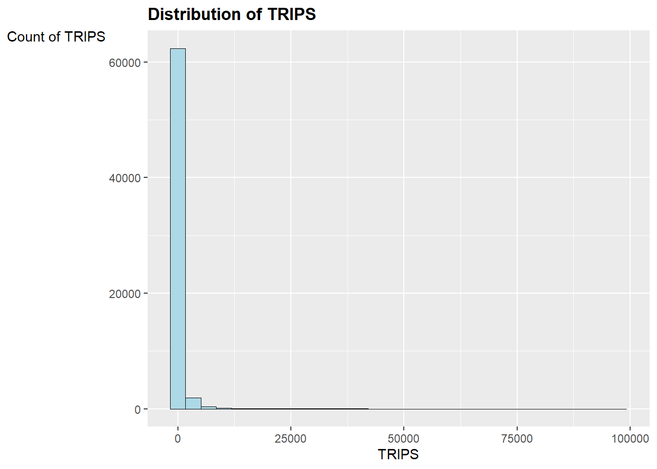

It seems to suggest that we should use a Poisson Regression Model.

Unconstrained Spatial Interaction Model

uncSIM <- glm(formula = TRIPS ~ 
                log(SCHOOL_COUNT) +
                log(BIZ_COUNT) +
                log(FINSERV_COUNT) +
                log(FOOD_COUNT) +
                log(POP) +
                log(TRAIN_EXITS_COUNT) +
                log(DESTIN_TRAIN_EXITS) +
                log(CHILDCARE_COUNT) +
                log(n_busstops) +
                log(DIST),
              family = poisson(link = "log"),
              data = inter_zonal_flow,
              na.action = na.exclude)

write_rds(uncSIM, "data/rds/uncSIM.rds")

uncSIM <- read_rds("data/rds/uncSIM.rds")

summary(uncSIM)

uncSIM$coefficients

            (Intercept)       log(SCHOOL_COUNT)          log(BIZ_COUNT) 
            15.33097167              0.23284279              0.06175043 
     log(FINSERV_COUNT)         log(FOOD_COUNT)                log(POP) 
             0.27830717             -0.28600788              0.10317452 
 log(TRAIN_EXITS_COUNT) log(DESTIN_TRAIN_EXITS)    log(CHILDCARE_COUNT) 
             0.15080169              0.47496463              0.23988144 
        log(n_busstops)               log(DIST) 
             0.29547319             -1.44671342

Based on the results, all the coefficients are statistically significant. The most influential explanatory variables are distance, destination train exit count and origin number of bus stops with coefficients of -1.45, 0.475 and 0.295 respectively.

Origin - Constrained Model

Note

For origin-constrained model, only explanatory variables representing the attractiveness at the destinations will be used.
All the explanatory variables including distance will be log transformed.
ORIGIN_Grid is used to model 𝜇_𝑖 . It must be in categorical data type.
It is important to note that -1 is added in the equation after the distance variable. The -1 serves the purpose of removing the intercept that by default, glm will insert into the model.

orcSIM <- glm(formula = TRIPS ~ 
                ORIGIN_Grid +
                log(SCHOOL_COUNT) +
                log(BIZ_COUNT) +
                log(FINSERV_COUNT) +
                log(FOOD_COUNT) +
                log(DESTIN_TRAIN_EXITS) +
                log(DIST) - 1,
              family = poisson(link = "log"),
              data = inter_zonal_flow,
              na.action = na.exclude)

write_rds(orcSIM, "data/rds/orcSIM.rds")

orcSIM <- read_rds("data/rds/orcSIM.rds")

tail(summary(orcSIM)$coefficients, n = 10)

Based on the results, all of the coefficients are statistically significant. The most influential explanatory variables are distance, destination train exit count and destination school count with coefficients of -1.5, 0.8 and 0.22 respectively.

Destination Constrained Model

Look at the propulsive variables.

decSIM <- glm(formula = TRIPS ~ 
                DESTIN_Grid +
                log(POP) +
                log(CHILDCARE_COUNT) +
                log(TRAIN_EXITS_COUNT) +
                log(n_busstops) +
                log(DIST) - 1,
              family = poisson(link = "log"),
              data = inter_zonal_flow,
              na.action = na.exclude)

write_rds(decSIM, "data/rds/decSIM.rds")

decSIM <- read_rds("data/rds/decSIM.rds")

tail(summary(decSIM)$coefficients, n = 10)

                         Estimate   Std. Error    z value Pr(>|z|)
DESTIN_Grid2405        17.5811819 5.002583e-03  3514.4207        0
DESTIN_Grid2406        14.5548014 2.397634e-02   607.0486        0
DESTIN_Grid2426        16.9283986 1.112556e-02  1521.5769        0
DESTIN_Grid2427        17.1907334 6.832253e-03  2516.1150        0
DESTIN_Grid2505        17.4420466 1.823257e-02   956.6424        0
log(POP)                0.1131565 8.436976e-05  1341.1971        0
log(CHILDCARE_COUNT)    0.2457757 3.667393e-04   670.1647        0
log(TRAIN_EXITS_COUNT)  0.2858289 3.261035e-04   876.4974        0
log(n_busstops)         0.2937858 5.204764e-04   564.4556        0
log(DIST)              -1.4849210 2.627804e-04 -5650.8062        0

Based on the results, all of the coefficients are statistically significant. The most influential explanatory variables are distance, origin number of bus stops and origin train exit count with coefficients of -1.48, 0.29 and 0.285 respectively.

Doubly Constrained Model

dbcSIM <- glm(formula = TRIPS ~ 
                ORIGIN_Grid + 
                DESTIN_Grid + 
                log(DIST),
              family = poisson(link = "log"),
              data = inter_zonal_flow,
              na.action = na.exclude)

write_rds (dbcSIM, "data/rds/dbcSIM.rds")

dbcSIM <- read_rds("data/rds/dbcSIM.rds")

tail(summary(dbcSIM)$coefficients, n = 10)

                  Estimate   Std. Error      z value      Pr(>|z|)
DESTIN_Grid2361 -0.4335822 0.0477142410    -9.087061  1.017526e-19
DESTIN_Grid2364 -2.4268487 0.0554825623   -43.740746  0.000000e+00
DESTIN_Grid2379 -1.4134320 0.0546363548   -25.869808 1.456682e-147
DESTIN_Grid2384  0.5506025 0.0473633047    11.625087  3.072801e-31
DESTIN_Grid2405  1.1919496 0.0471732041    25.267514 7.271724e-141
DESTIN_Grid2406 -1.8422643 0.0526903433   -34.963984 7.938991e-268
DESTIN_Grid2426  0.6352864 0.0482337535    13.170992  1.288934e-39
DESTIN_Grid2427  0.9464266 0.0473875928    19.972033  9.644730e-89
DESTIN_Grid2505  0.5333907 0.0507135194    10.517722  7.158336e-26
log(DIST)       -1.6077121 0.0002913633 -5517.894356  0.000000e+00

The variable distance is statistically significant.

Model Comparisons

We will use compare_performance() of performance package.

First of all, let us create a list called model_list by using the code chunk below.

model_list <- list(unconstrained=uncSIM,
                   originConstrained=orcSIM,
                   destinationConstrained=decSIM,
                   doublyConstrained=dbcSIM)

Next, we will compute the RMSE of all the models in model_list file by using the code chunk below.

compare_performance(model_list,
                    metrics = "RMSE")

# Comparison of Model Performance Indices

Name                   | Model |     RMSE
-----------------------------------------
unconstrained          |   glm | 1597.556
originConstrained      |   glm | 1470.300
destinationConstrained |   glm | 1396.745
doublyConstrained      |   glm | 1172.123

Goodness of Fit - Calculating RSquared Statistics

CalcRSquared <- function(observed, estimated){
  r <- cor(observed, estimated)
  R2 <- r^2
  R2
}

r_squared_values <- lapply(model_list, function(model) {
  observed_values <- model$data$TRIPS
  fitted_values <- model$fitted.values
  CalcRSquared(observed_values, fitted_values)
})

# Print the R-squared values for each model
print(r_squared_values)

$unconstrained
[1] 0.256333

$originConstrained
[1] 0.3696908

$destinationConstrained
[1] 0.4310837

$doublyConstrained
[1] 0.6000049

It seems that the Doubly Constrained Model is the best fitted across the four models, as compared to the other three. the RMSE of the Doubly Constrained Model is also the lowest.

Visualising the Fitted Values

Code

df <- as.data.frame(uncSIM$fitted.values) %>%
  round(digits = 0)

Code

SIM_data <- inter_zonal_flow %>%
  cbind(df) %>%
  rename(uncTRIPS = "uncSIM.fitted.values")

Code

df <- as.data.frame(orcSIM$fitted.values) %>%
  round(digits = 0)

Code

SIM_data <- SIM_data %>%
  cbind(df) %>%
  rename(orcTRIPS = "orcSIM.fitted.values")

Code

df <- as.data.frame(decSIM$fitted.values) %>%
  round(digits = 0)

Code

SIM_data <- SIM_data %>%
  cbind(df) %>%
  rename(decTRIPS = "decSIM.fitted.values")

Code

df <- as.data.frame(dbcSIM$fitted.values) %>%
  round(digits = 0)

Code

SIM_data <- SIM_data %>%
  cbind(df) %>%
  rename(dbcTRIPS = "dbcSIM.fitted.values")

write_rds(SIM_data, "data/rds/SIM_data.rds")

Code

unc_p <- ggplot(data = SIM_data,
                aes(x = uncTRIPS,
                    y = TRIPS)) +
  geom_point() +
  geom_smooth(method = lm)

orc_p <- ggplot(data = SIM_data,
                aes(x = orcTRIPS,
                    y = TRIPS)) +
  geom_point() +
  geom_smooth(method = lm)

dec_p <- ggplot(data = SIM_data,
                aes(x = decTRIPS,
                    y = TRIPS)) +
  geom_point() +
  geom_smooth(method = lm)

dbc_p <- ggplot(data = SIM_data,
                aes(x = dbcTRIPS,
                    y = TRIPS)) +
  geom_point() +
  geom_smooth(method = lm)

ggarrange(unc_p, orc_p, dec_p, dbc_p,
          ncol = 2,
          nrow = 2)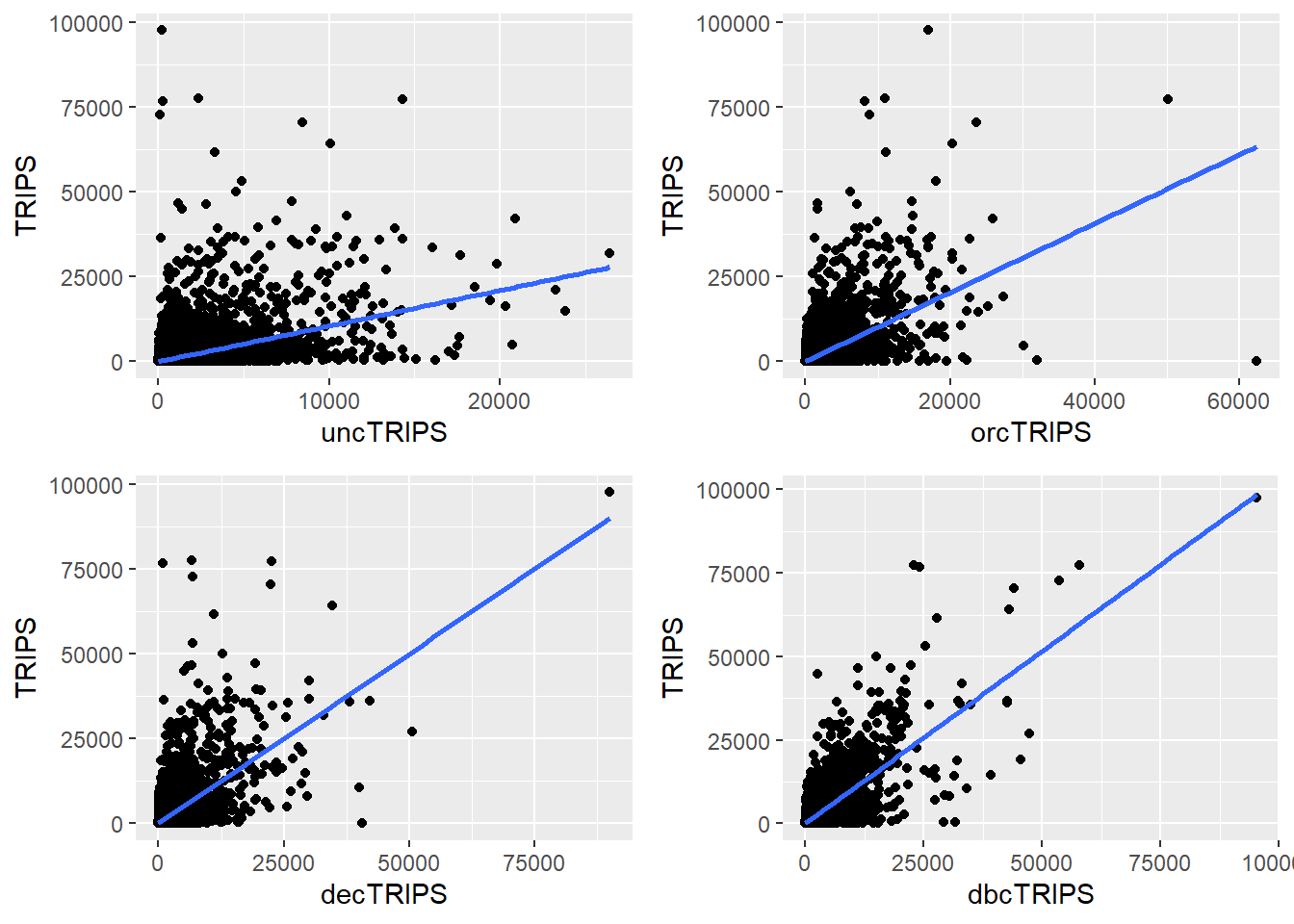

From the graphs - I noticed that as the number of trips increase, the fit is not as good. Additionally, there are quite a fair bit of variability in the data.

Limitations about Spatial Interaction Model

I realised that there are some limitations to the Spatial Interaction Models, namely:

The models are sensitive to distance - distance seems to be still the most influential factor in predicting the flow.
The models ignore the socio-economic factors of the population.
The models fail to explain the complex spatial patterns, e.g. accounting for the dependence between the hexagons, i.e. they are not independent.

Spatial Econometric Interaction Modelling (SEIM)

Since Prof talked about the SEIM in the class today, I want to see how we can use it for this take home ex 2.

Package Required

In this exercise, the development version (0.1.0.9010) of spflow will be used instead of the released version (0.1.0). The code chunk below will be used to install the development version of spflow package.

devtools::install_github("LukeCe/spflow")

pacman::p_load(tmap, sf, spdep, sp, Matrix,
               spflow, reshape2, knitr,
               tidyverse)

Data Preparation

Before we can calibrate Spatial Econometric Interaction Models by using spflow package, three data sets are required. They are:

a spatial weights,
a tibble data.frame consists of the origins, destination, flows and distances between the origins and destination, and
a tibble data.frame consists of the explanatory variables.

Our geographical data has already been built in the earlier segments and using the hexagonal grid.

Preparing the Weights Data

grid_busstops <- read_rds("data/rds/hexagon_busstop.rds")

centroids <- suppressWarnings({
    st_point_on_surface(st_geometry(hexagon_busstop))})

grid_nb <- list(
  "by_contiguity" = poly2nb(hexagon_busstop),
  "by_distance" = dnearneigh(centroids, 
                             d1 = 0, d2 = 5000),
  "by_knn" = knn2nb(knearneigh(centroids, 3))
)

Realised that there were data with zero neighbours. 3 data were removed.

nb_contiguity <- grid_nb$by_contiguity

nonzero_indices <- which(card(nb_contiguity) > 0)

hexagon_busstop <- hexagon_busstop %>% slice(nonzero_indices)

write_rds(grid_nb, "data/rds/grid_nb.rds")

Preparing the Flow Data

busstop_grid <- st_intersection(busstops, hexagon_grid_sf) %>%
  select(BUS_STOP_N, grid_id) %>%
  st_drop_geometry()

od_data <- left_join(odbus6_9 , busstop_grid,
            by = c("ORIGIN_PT_CODE" = "BUS_STOP_N")) %>%
  rename(ORIGIN_BS = ORIGIN_PT_CODE,
         ORIGIN_GRID = grid_id,
         DESTIN_BS = DESTINATION_PT_CODE)

duplicate <- od_data %>%
  group_by_all() %>%
  filter(n()>1) %>%
  ungroup()

od_data <- unique(od_data)

od_data <- left_join(od_data , busstop_grid,
            by = c("DESTIN_BS" = "BUS_STOP_N"))

od_data <- od_data %>%
  rename(DESTIN_GRID = grid_id) %>%
  drop_na() %>%
  group_by(ORIGIN_GRID, DESTIN_GRID) %>%
  summarise(TRIPS = sum(TRIPS))

write_rds(od_data, "data/rds/od_data.rds")

od_data <- read_rds("data/rds/od_data.rds")

busstop_grid_sp <- as(hexagon_busstop, "Spatial")

DISTANCE <- spDists(busstop_grid_sp, 
                    longlat = FALSE)

grid_names <- hexagon_busstop$grid_id

colnames(DISTANCE) <- paste0(grid_names)
rownames(DISTANCE) <- paste0(grid_names)

distPair <- melt(DISTANCE) %>%
  rename(DISTANCE = value)
head(distPair, 10)

distPair <- distPair %>%
  rename(ORIGIN_GRID = Var1,
         DESTIN_GRID = Var2)

flow_data <- distPair %>%
  left_join (od_data) %>%
  mutate(TRIPS = coalesce(TRIPS, 0))

write_rds(flow_data, "data/rds/grid_flow.rds")

Preparing the Variables Data

Using the data prepared in the earlier segments. But removing those with zero neighbours.

grid_var <- combined_data

grid_var <- grid_var %>% slice(nonzero_indices)

write_rds(grid_var, "data/rds/grid_var.rds")

Preparing spflow objects

grid_nb <- read_rds("data/rds/grid_nb.rds")
grid_flow <- read_rds("data/rds/grid_flow.rds")
grid_var <- read_rds("data/rds/grid_var.rds")

Three spflow objects are required, they are:

spflow_network-class, an S4 class that contains all information on a spatial network which is composed by a set of nodes that are linked by some neighborhood relation.
spflow_network_pair-class, an S4 class which holds information on origin-destination (OD) pairs. Each OD pair is composed of two nodes, each belonging to one network. All origin nodes must belong to the same origin network should be contained in one spflow_network-class, and likewise for the destinations.
spflow_network_multi-class, an S4 class that gathers information on multiple objects of types spflow_network-class and spflow_network_pair-class. Its purpose is to ensure that the identification between the nodes that serve as origins or destinations, and the OD-pairs is consistent (similar to relational data bases).

Creating `spflow_network-class` objects

spflow_network-class is an S4 class that contains all information on a spatial network which is composed by a set of nodes that are linked by some neighborhood relation. It can be created by using spflow_network() of spflow package.

For our model, we choose the contiguity based neighborhood structure.

grid_net <- spflow_network(
  id_net = "sg",
  node_neighborhood = nb2mat(grid_nb$by_contiguity),
  node_data = grid_var,
  node_key_column = "grid_id")

grid_net

Spatial network nodes with id: sg
--------------------------------------------------
Number of nodes: 831
Average number of links per node: 4.826
Density of the neighborhood matrix: 0.58% (non-zero connections)

Data on nodes:
    grid_id n_busstops SCHOOL_COUNT FOOD_COUNT FINSERV_COUNT POP
1        23          1            0          0             0   0
2        44          1            0          0             0   0
3        46          2            0          0             0   0
4        66          1            0          0             0   0
5        67          4            0          0             1   0
6        68          1            0          0             0   0
---     ---        ---          ---        ---           --- ---
826    2379          2            0          0             0   0
827    2384          4            0          0             0   0
828    2405          6            0          0             0   0
829    2406          4            0          0             0   0
830    2426          5            0          0             0   0
831    2427          3            0          0             2   0
    TRAIN_EXITS_COUNT CHILDCARE_COUNT BIZ_COUNT COORD_X COORD_Y
1                   0               0         0  103.62    1.27
2                   0               0         5  103.62    1.27
3                   0               0         4  103.62     1.3
4                   0               0         1  103.62    1.28
5                   0               0        50  103.62    1.29
6                   0               0        27  103.62     1.3
---               ---             ---       ---     ---     ---
826                 0               0         0  103.99    1.31
827                 0               0         1  103.99    1.37
828                 0               0         3     104    1.38
829                 0               0         0     104    1.39
830                 0               0         9     104    1.37
831                 0               0         1     104    1.38

Creating `spflow_network-class` object

spflow_network-class object is an S4 class which holds information on origin-destination (OD) pairs. Each OD pair is composed of two nodes, each belonging to one network. All origin nodes must belong to the same origin network should be contained in one spflow_network-class object and likewise for the destinations.

In spflow package, spflow_network_pair().

grid_net_pairs <- spflow_network_pair(
  id_orig_net = "sg",
  id_dest_net = "sg",
  pair_data = grid_flow,
  orig_key_column = "ORIGIN_GRID",
  dest_key_column = "DESTIN_GRID")

grid_net_pairs

Spatial network pair with id: sg_sg
--------------------------------------------------
Origin network id: sg (with 831 nodes)
Destination network id: sg (with 831 nodes)
Number of pairs: 690561
Completeness of pairs: 100.00% (690561/690561)

Data on node-pairs:
       DESTIN_GRID ORIGIN_GRID DISTANCE TRIPS
1               23          23        0     0
832             44          23      750     0
1663            46          23  3269.17     0
2494            66          23     1500     0
3325            67          23  2704.16     1
4156            68          23  3968.63     0
---            ---         ---      ---   ---
686406        2379        2427  7830.23     0
687237        2384        2427     1500  2238
688068        2405        2427      750  5329
688899        2406        2427      750    19
689730        2426        2427  1299.04     0
690561        2427        2427        0    10

Creating `spflow_network_multi-class` object

The sp_multi_network-class combines information on the nodes and the node-pairs and also ensures that both data sources are consistent. For example, if some of the origins in the sp_network_pair-class are not identified with the nodes in the sp_network_nodes-class an error will be raised.

spflow_network_multi()

grid_multi_net <-  spflow_network_multi(grid_net,
                                  grid_net_pairs)
grid_multi_net

Collection of spatial network nodes and pairs
--------------------------------------------------
Contains 1 spatial network nodes  
    With id :  sg
Contains 1 spatial network pairs  
    With id :  sg_sg

Availability of origin-destination pair information:

 ID_ORIG_NET ID_DEST_NET ID_NET_PAIR COMPLETENESS       C_PAIRS  C_ORIG  C_DEST
          sg          sg       sg_sg      100.00% 690561/690561 831/831 831/831

plot(mpsz$geometry)

spflow_map(
  grid_multi_net,
  flow_var = "TRIPS",
  add = TRUE, 
  legend_position = "bottomleft",
  filter_lowest = .99999, 
  remove_intra = TRUE,
  cex = 1)

Model Calibration

The core function of the package is spflow(). It provides an interface to three different estimators of spatial econometric interaction models (Dargel 2021) that allow the user to estimate origin-destination flows with spatial autocorrelation.

The three different estimators currently supported by spflow are:

Maximum Likelihood Estimation (MLE) which is the default estimation procedure. The matrix form estimation in the framework of this model was first developed by LeSage and Pace (2008) and then improved by Dargel (2021) . Spatial two-stage least squares (S2SLS)
Spatial Two-stage Least Squares (S2SLS) estimator is an adaptation of the one proposed by Kelejian and Prucha (1998), to the case of origin-destination flows, with up to three neighborhood matrices Dargel (2021). A similar estimation is done by Tamesue and Tsutsumi (2016). The user can activate the S2SLS estimation via the estimation_control argument using the input spflow_control(estimation_method = "s2sls").
Bayesian Markov Chain Monte Carlo (MCMC) estimator is based on the ideas of LeSage and Pace (2009) and incorporates the improvements proposed in Dargel (2021) . The estimation is based on a tuned Metropolis-Hastings sampler for the auto-regressive parameters, and for the remaining parameters it uses Gibbs sampling. The routine uses 5500 iterations of the sampling procedure and considers the first 2500 as burn-in period. The user can activate the S2SLS estimation via the estimation_control argument using the input spflow_control(estimation_method = "mcmc").

Estimation with default settings requires two arguments: an sp_multi_network-class and a flow_formula. The flow_formula specifies the model we want to estimate. The function offers a formula interface adapted to spatial interaction models, which has the following structure: Y ~ O_(X1) + D_(X2) + I_(X3) + P_(X4). This structure reflects the different data sources involved in such a model. On the left hand side there is the independent variable Y which corresponds to the vector of flows. On the right hand side we have all the explanatory variables. The functions O_(…) and D_(…) indicate which variables are used as characteristics of the origins and destinations respectively. Similarly, I_(…) indicates variables that should be used for the intra-regional parameters. Finally, P_(…) declares which variables describe origin-destination pairs, which most frequently will include a measure of distance.

All the declared variables must be available in the provided spflow_network_multi() object, which gathers information on the origins and destinations (inside spflow_network() objects), as well as the information on the origin-destination pairs (inside a spflow_network_pair() object).

Using the short notation Y ~ . is possible and will be interpreted as usual, in the sense that we use all variables that are available for each data source. Also mixed formulas, such as Y ~ . + P_(log(X4) + 1), are possible. When the dot shortcut is combined with explicit declaration, it will only be used for the non declared data sources.

Using Model Control

spflow_formula <- log(1 + TRIPS) ~ 
    O_(n_busstops +
    TRAIN_EXITS_COUNT + 
    FOOD_COUNT +
    POP +
    CHILDCARE_COUNT) +
    D_(SCHOOL_COUNT +
    BIZ_COUNT +
    FINSERV_COUNT +
    n_busstops) +
    P_(log(DISTANCE + 1))

model_control <- spflow_control(
  estimation_method = "mle",
  model = "model_8")

mle_model8 <- spflow(
  spflow_formula,
  spflow_networks = grid_multi_net,
  estimation_control = model_control)

mle_model8

--------------------------------------------------
Spatial interaction model estimated by: MLE  
Spatial correlation structure: SDM (model_8)
Dependent variable: log(1 + TRIPS)

--------------------------------------------------
Coefficients:
                             est     sd    t.stat  p.val
rho_d                      0.677  0.001   565.504  0.000
rho_o                      0.663  0.001   543.027  0.000
rho_w                     -0.449  0.001  -407.063  0.000
(Intercept)                0.806  0.013    61.639  0.000
(Intra)                   -0.723  0.026   -27.305  0.000
D_SCHOOL_COUNT             0.001  0.001     1.074  0.283
D_SCHOOL_COUNT.lag1        0.007  0.003     2.602  0.009
D_BIZ_COUNT                0.000  0.000     0.923  0.356
D_BIZ_COUNT.lag1           0.000  0.000     2.869  0.004
D_FINSERV_COUNT            0.004  0.000    33.258  0.000
D_FINSERV_COUNT.lag1      -0.001  0.000    -8.567  0.000
D_n_busstops               0.010  0.000    34.871  0.000
D_n_busstops.lag1         -0.009  0.001   -17.052  0.000
O_n_busstops               0.009  0.000    31.563  0.000
O_n_busstops.lag1         -0.008  0.001   -14.450  0.000
O_TRAIN_EXITS_COUNT        0.014  0.001    22.402  0.000
O_TRAIN_EXITS_COUNT.lag1  -0.017  0.001   -14.768  0.000
O_FOOD_COUNT               0.000  0.000     2.437  0.015
O_FOOD_COUNT.lag1          0.001  0.000     4.038  0.000
O_POP                      0.000  0.000     4.374  0.000
O_POP.lag1                 0.000  0.000    -0.637  0.524
O_CHILDCARE_COUNT          0.003  0.001     5.961  0.000
O_CHILDCARE_COUNT.lag1     0.001  0.001     0.946  0.344
P_log(DISTANCE + 1)       -0.086  0.001   -65.968  0.000

--------------------------------------------------
R2_corr: 0.718472  
Observations: 690561  
Model coherence: Unknown

The R2 is 0.718 which is higher compared to the previous models done in Spatial Interaction Models. Will examining the variables further:

	est	sd	t.stat	p.val	Remarks
rho_d	0.677	0.001	565.502	0.000
rho_o	0.663	0.001	543.029	0.000
rho_w	-0.449	0.001	-407.064	0.000
(Intercept)	0.806	0.013	61.639	0.000
(Intra)	-0.723	0.026	-27.305	0.000
D_SCHOOL_COUNT	0.001	0.001	1.074	0.283	Surprisingly - this is not statistically significant.
D_SCHOOL_COUNT.lag1	0.007	0.003	2.602	0.009
D_BIZ_COUNT	0.000	0.000	0.923	0.356	Surprisingly - this is not statistically significant.
D_BIZ_COUNT.lag1	0.000	0.000	2.869	0.004
D_FINSERV_COUNT	0.004	0.000	33.258	0.000
D_FINSERV_COUNT.lag1	-0.001	0.000	-8.567	0.000
D_n_busstops	0.010	0.000	34.871	0.000
D_n_busstops.lag1	-0.009	0.001	-17.052	0.000
O_n_busstops	0.009	0.000	31.563	0.000
O_n_busstops.lag1	-0.008	0.001	-14.450	0.000
O_TRAIN_EXITS_COUNT	0.014	0.001	22.403	0.000
O_TRAIN_EXITS_COUNT.lag1	-0.017	0.001	-14.768	0.000
O_FOOD_COUNT	0.000	0.000	2.437	0.015	Surprisingly - this is statistically significant. But the t.stat is rather low.
O_FOOD_COUNT.lag1	0.001	0.000	4.038	0.000
O_POP	0.000	0.000	4.374	0.000
O_POP.lag1	0.000	0.000	-0.637	0.524
O_CHILDCARE_COUNT	0.003	0.001	5.961	0.000	Surprisingly - this is statistically significant. But the t.stat is rather low.
O_CHILDCARE_COUNT.lag1	0.001	0.001	0.946	0.344
P_log(DISTANCE + 1)	-0.086	0.001	-65.968	0.000

It sseems to suggest that travel is still very much explained by the number of bus stops within that area, the number of train station exits at that area and that there are certain type of industry, such as FINSERV that will see most of the people travelling to by bus etc.

Looking at the multi-collinearity:

corr_residual <- pair_cor(mle_model8)
colnames(corr_residual) <- substr(colnames(corr_residual),1,3)
cor_image(corr_residual, cex = 0.5)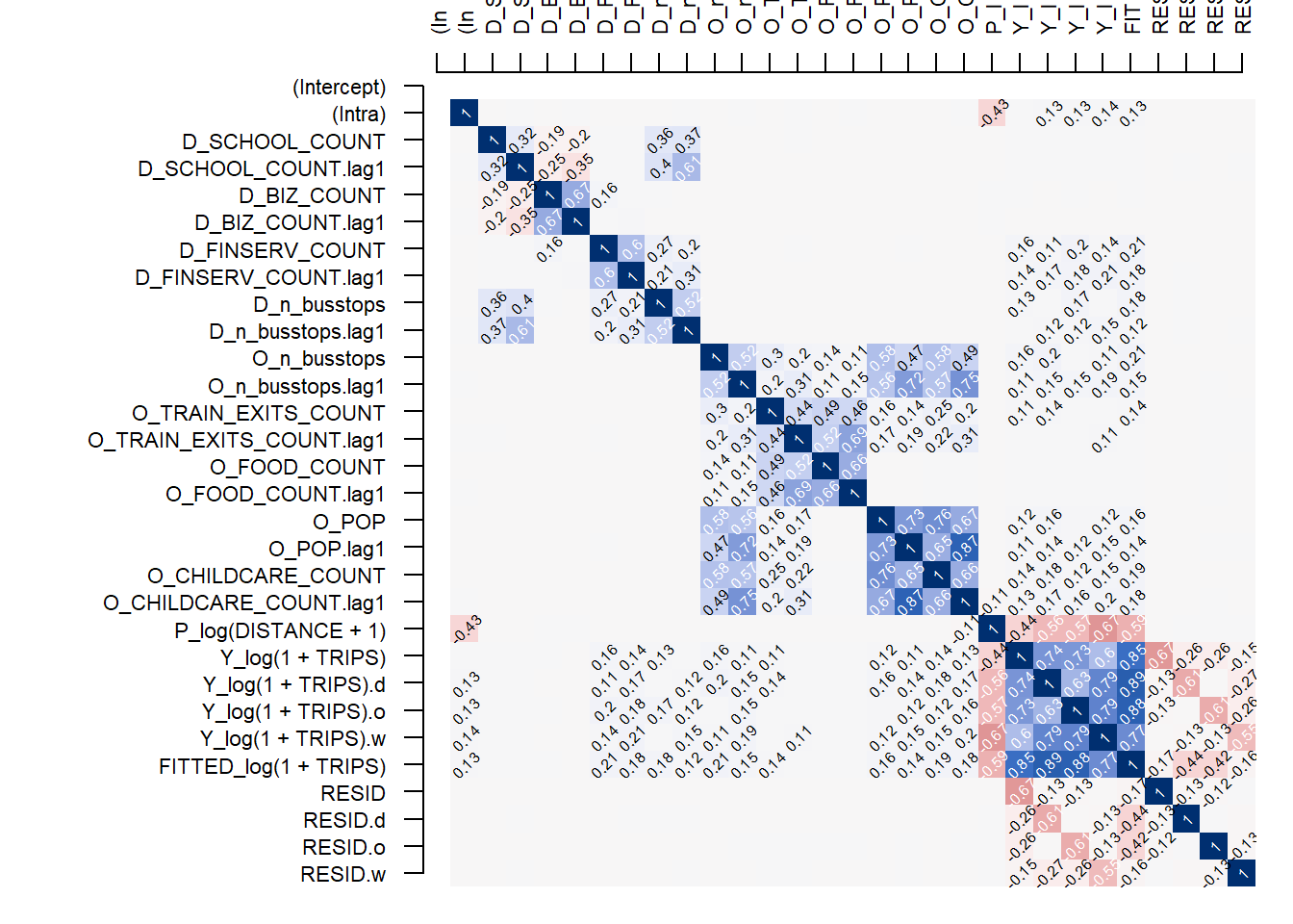

old_par <- par(mfrow = c(1, 3), 
               mar = c(2,2,2,2))
spflow_moran_plots(mle_model8)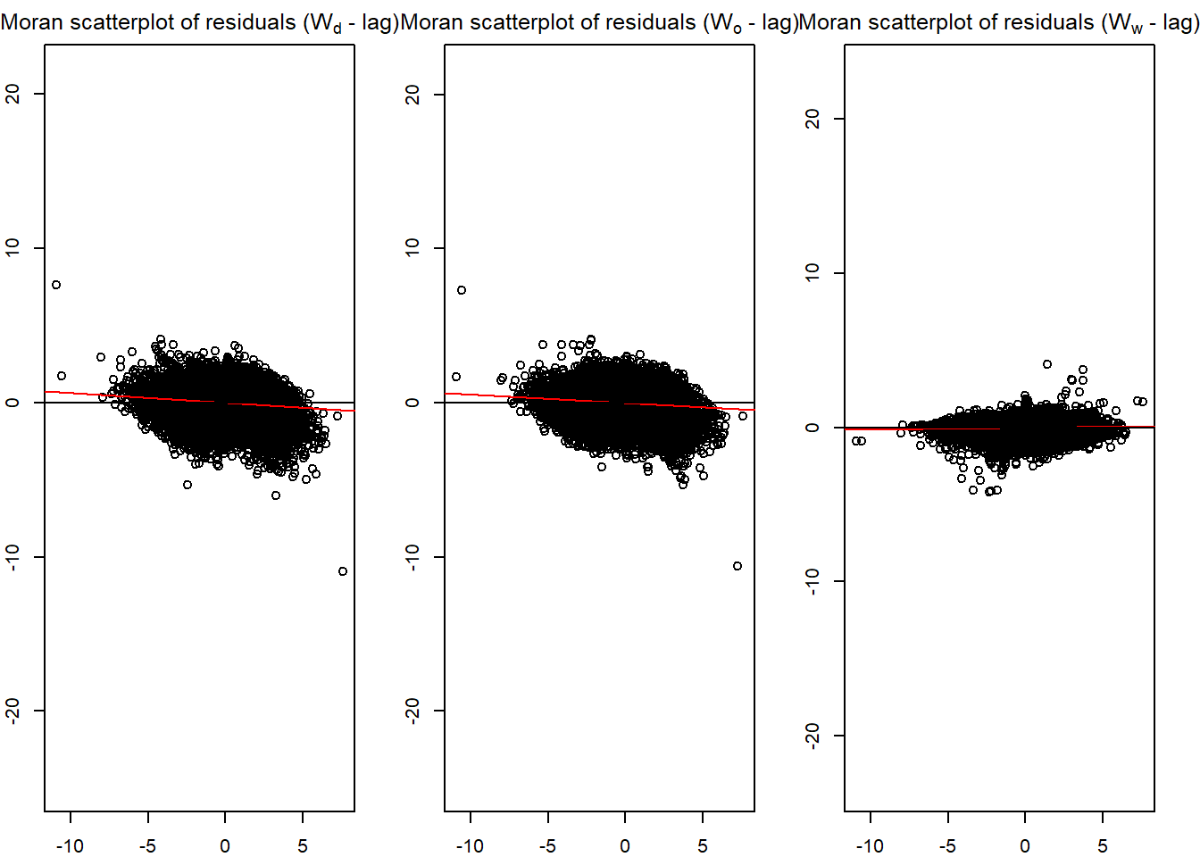

Conclusion

It seems that the Spatial Econometric Interaction Modelling did a better job in fitting the data. However, i would still need to further examine it and look at the other models as well. Submitting this portion first due to time constraint.

Nonetheless - I think I have learnt a lot during this course, not just about geospatial analytics, but also about the various tools that we can used to get data. It is certainly useful for us in the future.

Would like to thank Prof Kam for putting in so much effort in this short five weeks.

Overview of the Exercise

Open Gov Data

Specially collected data

Getting Started

Loading the Packages

Preparing the Flow Data

Write/Read Data into rds for Subsequent Usage

Visualising the Spatial Interaction

Analysis of Spatial Flow

Spatial Patterns

Attractiveness Variables

Propulsive Variables

Preparing the Data on Populace

Train Station Exit

Location of Pre-Schools

Visualising the Flow with the Variables

Spatial Interaction Modelling

Computing the Distance Matrix

Preparing the Flow Data

Grouping the Flow Data

Separating the Intra-Flow Data

Combining Passenger Volume Data with Dist Data

Combining the Data with Propulsive and Attractive Variables Data

Calibrating Spatial Interaction Models

Basic Plot of the Inter Zonal Flow Data

Unconstrained Spatial Interaction Model

Origin - Constrained Model

Destination Constrained Model

Doubly Constrained Model

Model Comparisons

Goodness of Fit - Calculating RSquared Statistics

Visualising the Fitted Values

Limitations about Spatial Interaction Model

Spatial Econometric Interaction Modelling (SEIM)

Package Required

Data Preparation

Preparing the Weights Data

Preparing the Flow Data

Preparing the Variables Data

Preparing spflow objects

Creating spflow_network-class objects

Creating spflow_network-class object

Creating spflow_network_multi-class object

Model Calibration

Using Model Control

Conclusion

Creating `spflow_network-class` objects

Creating `spflow_network-class` object

Creating `spflow_network_multi-class` object