pacman::p_load(tmap, sf, DT, stplanr, performance, ggpubr, tidyverse)Hands-On Ex 3
Processsing and Visualising Flow Data
Loading the required Packages
Here’s a brief overview of each of the R packages:
tmap: A package for thematic mapping and spatial visualization. It provides a flexible and powerful framework for creating static and interactive maps.sf: A package for simple features in R. It provides a standard for representing and manipulating spatial vector data. It allows you to work with spatial data using a tidy data structure.DT: An interactive data table package. It allows you to create interactive and customizable data tables in R, which can be particularly useful for exploring and presenting data.stplanr: A package for transport planning. It provides functions for spatial transport planning and analysis, including route planning, isochrones, and accessibility analysis.performance: A package for assessing and evaluating the performance of predictive models. It includes functions for model evaluation, comparison, and visualization.ggpubr: A package for creating complex and customized plots usingggplot2. It enhancesggplot2functionalities and provides functions for creating publication-ready graphics.tidyverse: A collection of R packages designed for data science. It includes a set of packages (e.g.,dplyr,ggplot2,tidyr, etc.) that work seamlessly together, promoting a tidy data workflow.
Preparing the Flow Data
We will be using the Passenger Volume data from LTA again.
We will be using the data from Oct 23.
odbus <- read_csv("data/aspatial/origin_destination_bus_202310.csv")glimpse (odbus)Rows: 5,694,297
Columns: 7
$ YEAR_MONTH <chr> "2023-10", "2023-10", "2023-10", "2023-10", "2023-~
$ DAY_TYPE <chr> "WEEKENDS/HOLIDAY", "WEEKDAY", "WEEKENDS/HOLIDAY",~
$ TIME_PER_HOUR <dbl> 16, 16, 14, 14, 17, 17, 17, 7, 14, 14, 10, 20, 20,~
$ PT_TYPE <chr> "BUS", "BUS", "BUS", "BUS", "BUS", "BUS", "BUS", "~
$ ORIGIN_PT_CODE <chr> "04168", "04168", "80119", "80119", "44069", "2028~
$ DESTINATION_PT_CODE <chr> "10051", "10051", "90079", "90079", "17229", "2014~
$ TOTAL_TRIPS <dbl> 3, 5, 3, 5, 4, 1, 24, 2, 1, 7, 3, 2, 5, 1, 1, 1, 1~odbus$ORIGIN_PT_CODE <- as.factor(odbus$ORIGIN_PT_CODE)
odbus$DESTINATION_PT_CODE <- as.factor(odbus$DESTINATION_PT_CODE) For the purpose of the study, we will be looking at the data from 6 am to 9am, weekdays.
odbus6_9 <- odbus %>%
filter(DAY_TYPE == "WEEKDAY") %>%
filter(TIME_PER_HOUR >= 6 &
TIME_PER_HOUR <= 9) %>%
group_by(ORIGIN_PT_CODE,
DESTINATION_PT_CODE) %>%
summarise(TRIPS = sum(TOTAL_TRIPS))
datatable(odbus6_9)write_rds(odbus6_9, "data/rds/odbus6_9.rds")The code chunk below will be used to import the save odbus6_9.rds into R environment.
odbus6_9 <- read_rds("data/rds/odbus6_9.rds")For the purpose of this exercise, two geospatial data will be used. They are:
BusStop: This data provides the location of bus stop as at last quarter of 2022.
MPSZ-2019: This data provides the sub-zone boundary of URA Master Plan 2019.
Both data sets are in ESRI shapefile format.
busstop <- st_read(dsn = "data/geospatial",
layer = "BusStop") %>%
st_transform(crs = 3414)Reading layer `BusStop' from data source
`C:\zjjgithubb\ISSS624\HandsOnEx\HandsOnEx3\data\geospatial'
using driver `ESRI Shapefile'
Simple feature collection with 5161 features and 3 fields
Geometry type: POINT
Dimension: XY
Bounding box: xmin: 3970.122 ymin: 26482.1 xmax: 48284.56 ymax: 52983.82
Projected CRS: SVY21mpsz <- st_read(dsn = "data/geospatial",
layer = "MPSZ-2019") %>%
st_transform(crs = 3414)Reading layer `MPSZ-2019' from data source
`C:\zjjgithubb\ISSS624\HandsOnEx\HandsOnEx3\data\geospatial'
using driver `ESRI Shapefile'
Simple feature collection with 332 features and 6 fields
Geometry type: MULTIPOLYGON
Dimension: XY
Bounding box: xmin: 103.6057 ymin: 1.158699 xmax: 104.0885 ymax: 1.470775
Geodetic CRS: WGS 84busstop_mpsz <- st_intersection(busstop, mpsz) %>%
select(BUS_STOP_N, SUBZONE_C) %>%
st_drop_geometry()write_rds(busstop_mpsz, "data/rds/busstop_mpsz.rds") od_data <- left_join(odbus6_9 , busstop_mpsz,
by = c("ORIGIN_PT_CODE" = "BUS_STOP_N")) %>%
rename(ORIGIN_BS = ORIGIN_PT_CODE,
ORIGIN_SZ = SUBZONE_C,
DESTIN_BS = DESTINATION_PT_CODE)duplicate <- od_data %>%
group_by_all() %>%
filter(n()>1) %>%
ungroup()od_data <- unique(od_data)od_data <- left_join(od_data , busstop_mpsz,
by = c("DESTIN_BS" = "BUS_STOP_N"))
duplicate <- od_data %>%
group_by_all() %>%
filter(n()>1) %>%
ungroup()
od_data <- unique(od_data)
od_data <- od_data %>%
rename(DESTIN_SZ = SUBZONE_C) %>%
drop_na() %>%
group_by(ORIGIN_SZ, DESTIN_SZ) %>%
summarise(MORNING_PEAK = sum(TRIPS))write_rds(od_data, "data/rds/od_data.rds")
od_data <- read_rds("data/rds/od_data.rds")Visualising the Spatial Interaction
We will be using the stplanr package.
stplanr was initially developed to answer a practical question: how to convert official data on travel behaviour into geographic objects that can be plotted on a map and analysed using methods from geographical information systems (GIS)? Specifically, how can origin-destination (OD) data, such as the open datasets provided by the UK Data Services WICID portal (see wicid.ukdataservice.ac.uk/), be used to estimate cycling potential down to the street levels at city and national levels? The project was initially developed to support the Propensity to Cycle Tool (PCT), which has now been deployed as a national web application hosted at www.pct.bike and written-up as an academic paper (Lovelace et al. 2017).
stplanr has since grown to include a wide range of functions for transport planning. The package was reviewed through the rOpenSci package review process and the package is now hosted on their site. See the website at docs.ropensci.org/stplanr. A more detailed overview of the package’s aims and capabilities is contained in a longer vignette, which has since been published in the R Journal (Lovelace and Ellison 2018).
Removing Intra-zonal Flows
We will not plot the intra-zonal flows. The code chunk below will be used to remove intra-zonal flows.
od_data1 <- od_data[od_data$ORIGIN_SZ!=od_data$DESTIN_SZ,]Creating desire lines
In this code chunk below, od2line() of stplanr package is used to create the desire lines.
flowLine <- od2line(flow = od_data1,
zones = mpsz,
zone_code = "SUBZONE_C")Visualising the Desire Lines
sf::st_geometry(mpsz)Geometry set for 332 features
Geometry type: MULTIPOLYGON
Dimension: XY
Bounding box: xmin: 2667.538 ymin: 15748.72 xmax: 56396.44 ymax: 50256.33
Projected CRS: SVY21 / Singapore TM
First 5 geometries:sf::st_geometry(flowLine)Geometry set for 20787 features
Geometry type: LINESTRING
Dimension: XY
Bounding box: xmin: 5105.594 ymin: 25813.33 xmax: 49483.22 ymax: 49552.79
Projected CRS: SVY21 / Singapore TM
First 5 geometries:tmap_mode("plot")
tm_shape(mpsz) +
tm_borders() +
tm_polygons() +
tm_shape(flowLine) +
tm_lines(lwd = "MORNING_PEAK",
style = "quantile",
scale = c(0.1, 1, 3, 5, 7, 10),
n = 6,
alpha = 0.3)
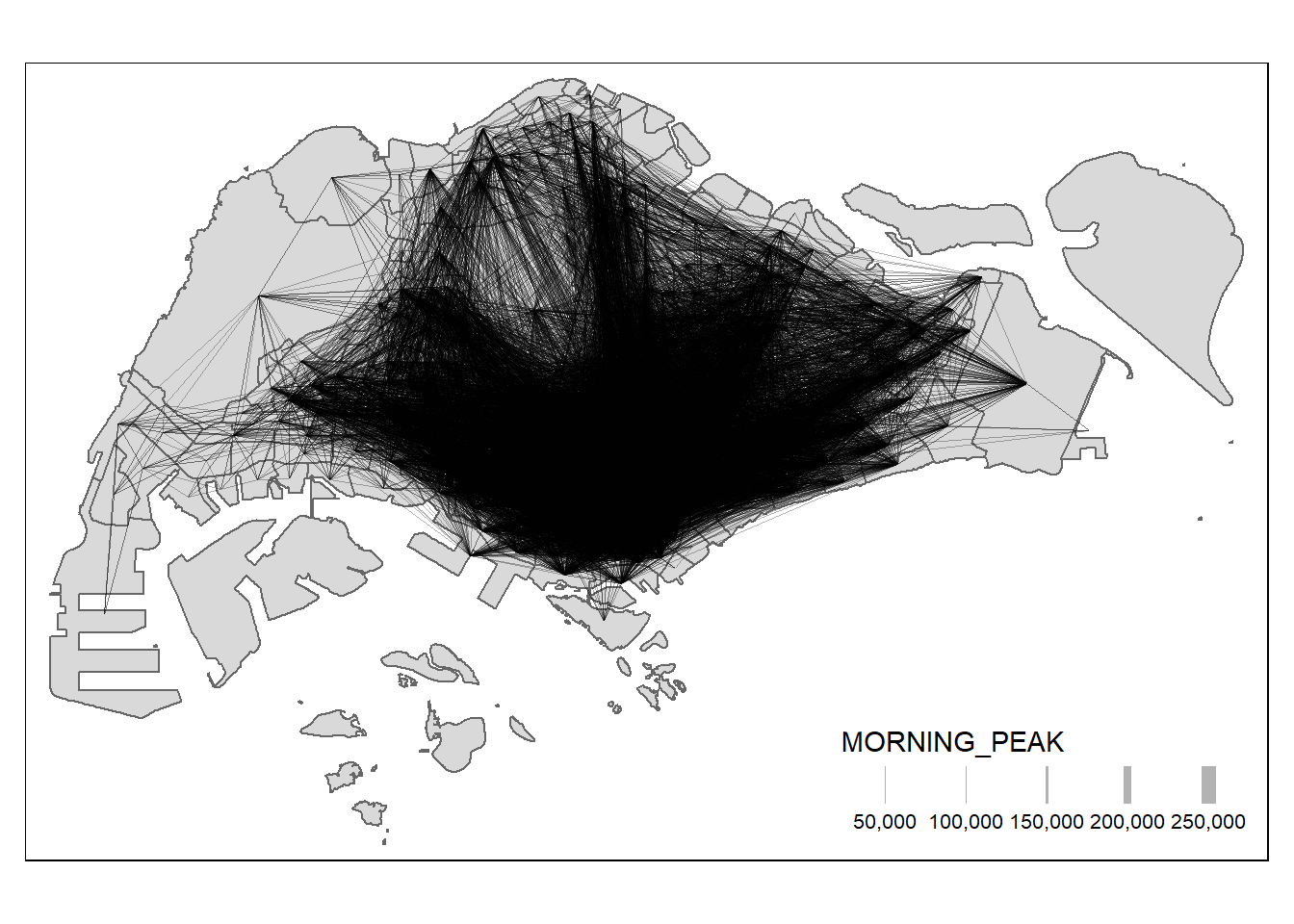
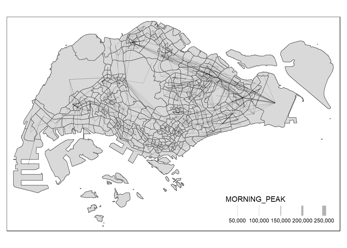
When the flow data are very messy and highly skewed like the one shown above, it is wiser to focus on selected flows, for example flow greater than or equal to 5000 as shown below.
tmap_mode("plot")
tm_shape(mpsz) +
tm_borders() +
tm_polygons() +
flowLine %>%
filter(MORNING_PEAK >= 5000) %>%
tm_shape() +
tm_lines(lwd = "MORNING_PEAK",
style = "quantile",
scale = c(0.1, 1, 3, 5, 7, 10),
n = 6,
alpha = 0.3)